API: auxiliary classes

Code author: Frédéric Richard <frederic.richard_at_univ-amu.fr>

Periodic functions (perfunction)

class afbf.Classes.PeriodicFunction.perfunction(ftype='step-smooth', param=0, fname='noname')

Bases: object

This class handles \(\pi\)-periodic positive parametric functions.

The available function representations are

the representation in a Fourier basis,
a representation by step functions,
a representation by smoothed step functions.

In the Fourier representation, the function is defined as

\[f(t) = a_0 + \sum_{m=1}^M a_{m, 1} \cos(2mt)+a_{m, 2} \sin(2mt),\]

where \(a_0\) and \(a_{m, k}\) are real parameters.

A step function is defined as

\[f(t) = a_0 \left( \delta_{[-\frac{\pi}{2}, \psi_1)}(t) + \delta_{[\psi_{M+1}, \frac{\pi}{2})}(t) \right) + \sum_{m=1}^M a_i \delta_{[\psi_i, \psi_{i+1})}(t),\]

where \(a_i\) are non-negative parameters, and \(\psi_i\) are ordered angles in \([-\frac{\pi}{2}, \frac{\pi}{2})\).

The definition of step functions can be adapted to include smooth transitions between intervals where the function is constant.

Note

Representations are defined by an expansion of the form

\[f(t) = \sum_{m=0}^M \alpha_m B_m(t)\]

for some coefficients \(\alpha_m\) and basis functions \(B_m\).

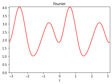
Example:: Definition of a function using the Fourier representation with \(M=3\) (i.e. 7 coefficients).

from afbf import perfunction
f1 = perfunction('Fourier', 3, 'Fourier')
f1.Display(1)

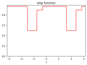
Example:: Definition of a function with three steps.

from afbf import perfunction
f2 = perfunction('step', 3, 'step function')
f2.Display(2)

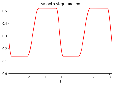
Example:: Definition of a smooth function with two steps.

from afbf import perfunction
f3 = perfunction('step-smooth', 2, 'smooth step function')
f3.Display(3)

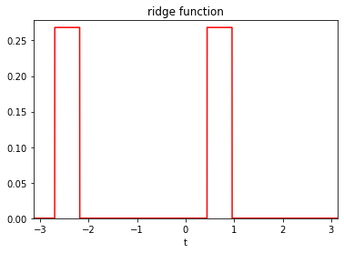
Example:: Definition of a step function with a ridge.

from afbf import perfunction
f4 = perfunction('ridge-step', 1, 'ridge function')
f4.Display(4)

Parameters:

fname (str) – Name of the function.
ftype (str) –
Type of the function representation. Some predefined type are available:
- ’step’: step function.
- ’step-constant’: constant function.
- ’step-ridge’: a step function with ridges.
- ’step-smooth’: smooth step function.
- ’Fourier’: Fourier representation.
fparam (ndarray) – Representation parameters \(\alpha_m\).
finter (ndarray) – Interval bounds \(\psi_i\) for a step function.
steptrans (boolean) – True if there are transitions between step.
trans (int) – indicate where step transitions are on even or odd intervals ({0, 1}).
basis (ndarray) – an array where values of the mth basis function \(B_m\) of the representation are on the mth row.
t (ndarray) – positions at which to evaluate the function.
stats (ndarray) – Basics statistics; min, max, mean, median of the function.
dev (ndarray) – Measures of deviations of the function; standard deviation, absolute deviations to the mean and to the median.
sharpness (ndarray) – Measures of sharpness computed on discrete function derivative (discrete tv-norm, maximum of absolute discrete derivative).
smode – Simulation mode of a step function (see SetStepSampleMode).
translate (float) – Translation to be applied to the function (defaut to 0).
rescale (float) – Factor of a rescaling to be applied to the function.

ApplyTransforms(translate=None, rescale=None)

Apply translation and/or rescaling transform to the function.

Parameters:

translate (float) – Translation.
rescale (float) – scaling factor (must be positive).

Returns:

Attributes translate, rescale.

ChangeParameters(fparam=None, finter=None)

Change parameters of the function while keeping its representation.

If parameters are not given, the parameters are changed at random.

Parameters:

fparam (ndarray, optional.) – Parameters of the function. The default is None.
finter (ndarray, optional) – Step interval bounds (only for step functions). The default is None.

Returns:

Attributes fparam.

CheckValidity()

Check the validity of the periodic function.

Returns:: True if attributes are properly defined.
Return type:: boolean

ComputeFeatures(m=10000)

Compute some features describing the function.

Parameters:: m (int, optional) – Number of discrete positions to evaluate the function. Default to 10000.
Returns:: Precision of the evaluation.
Rtypes:: scalar
Returns:: Attributes stats, dev, sharpness.

ComputeFourierBasis()

Compute basis functions of the Fourier representation.

Returns:: Attribute basis.

ComputeStepBasis()

Compute basis functions of a representation by a step function at positions given in attribute t.

Returns:: Attribute basis.

Display(nfig=1)

Plot the graph of the function.

Parameters:: nfig (int, optional) – The index of the figure. Default to 1.

Evaluate(t=None)

Evaluate the function at some positions.

Parameters:: t (ndarray, optional.) – Positions at which the function is computed.
Returns:: Attribute values.

Note

If parameter t is omitted, the function is evaluated at points of the previous call of the function.

InitFourierFunction(mode='init', M=3)

Define or update the Fourier representation of a periodic function.

Parameters:

mode (str, optional) – The utilisation mode (‘init’, ‘update’). Use the ‘init’ mode to set the function representation at random (default), or ‘update’ to change its parameters at random. The default is ‘init’.
M (int, optional) – M * 2 + 1 is the number of Fourier coefficients. The default is 3.

Returns:

Attribute fparam.

InitStepFunction(ftype='step-constant', mode='init', M=2)

Define or update a step function at random.

Parameters:

ftype (str, optional) – The type of step function. (‘step’,’step-constant’,’step-ridge’,’step-smooth’). The default is ‘step-constant’.
mode (str, optional) – The utilisation mode (‘init’, ‘update’). The default is ‘init’.
M (int, optional) – Number of steps. The default is 2.

Returns:

Attributes fparam, finter.

SampleFourierCoefficients()

Sample the Fourier coefficients.

Returns:: Attribute fparam.

SampleStepConstants(k=-1)

Sample constants within (0, 1).

Parameters:: k (int, optional) – index where to put the minimal value. The default is -1.
Returns:: Attribute fparam.

Note

The simulation of the step constants depends on the attribute smode:

smode[0]=’unif’:
step values are sampled from a uniform distribution on (smode[1], smode[2]).

smode[0]=’unifmin’:
the minimal step value is sampled from a uniform distribution on (smode[1], smode[2]).

smode[0]=’unifrange’:
the step value range is sampled from a uniform distribution on (0, smode[2] - smode[1]).

The mode of simulation can be changed using SetStepSampleMode.

SampleStepIntervals()

Sample interval bounds of a step function.

Returns:: The index of the interval whose size is uniformly sampled.
Return type:: int

Note

The simulation of the step constants depends on the attribute smode:

smode[3]=’unif’:
the bounds are uniformly sampled over the interval (-pi/2, pi/2).

smode[3]=’nonunif’:
the bounds are sampled so that the size of one of them is uniformly sampled.

smode[4] is a minimal interval size.

The mode of simulation can be changed using SetStepSampleMode.

Save(filename)

Save a periodic function in a file.

Parameters:: filename (str.) – address of the file.

Note

The function can be rebuilt using the function LoadPerfunction.

SetStepSampleMode(mode_cst='unif', a=0, b=1, mode_int='unif', d=0)

Set the simulation mode for sampling parameters of a step function.

Parameters:

mode_cst (str, optional) –
The mode of simulation of constants \(a_m\):
- if mode_cst = ‘unif’:
  step values are sampled from a uniform distribution on (a, b).
- if mode_cst = ‘unifmin’:
  the minimal step value is sampled from a uniform distribution on (a, b).
- if mode_cst = ‘unifrange’:
  the step value range is sampled from a uniform distribution on (a, b).
The default is ‘unif’.
a (float, optional) – lower bound. The default is 0.
b (float, optional) – upper bound. The default is 1.
mode_int (str, optional) –
The mode of simulation of interval bounds \(\psi_m\):
- if mode_int=’unif’:
  the bounds are uniformly sampled over the interval (-pi/2, pi/2).
- if mode_int=’nonunif’:
  the bounds are sampled so that the size of one of them is uniformly sampled.
The default is ‘unif’.
d (float, optional) – Minimal value of interval size. The default is 0.

Returns:

Attribute smode.

SetUniformStepInterval()

Set uniform step intervals.

Returns:: Attribute finter, trans.

ShowParameters(): Show the parameters of the function.

Coordinates (coordinates)

class afbf.Classes.SpatialData.coordinates(N=-1)

Bases: object

This class handles a set of coordinates in the plane.

Coordinates are pairs (x, y) of integers referring to a plane position (x / N, y / N). Set of coordinates can either be on a uniform grid or at arbitrary positions.

A uniform grid is defined as \([\![1, N]\!] \times [\![1, N]\!]\). It can also be signed, in which case it is of the form \([\![1, N]\!] \times [\![-N, N]\!]\).

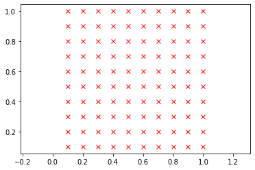
Example:: Define and display a grid of size 10 x 10.

from afbf import coordinates
coord = coordinates(10)
coord.Display(1)

Parameters:

xy (ndarray of shape (ncoord, 2)) – set of Cartesian coordinates; xy[m, :] are the mth coordinates.
N (int) – Factor to be applied to coordinates.
Nx (int) – Grid dimension: number of x coordinates.
Ny (int) – Grid dimension: number of y coordinates.
grid (bool) – True if grid coordinates.

ApplyAffineTransform(A)

Apply an affine transform A to coordinates.

Given a matrix \(A\) of shape (2, 2) and coordinates \((x, y)\), the transform is defined as

\[(\tilde x, \tilde y) = (x, y) A.\]

Parameters:: A (ndarray) – An array of shape (2, 2) of type int defining the affine transform.
Returns:: Attributes xy.
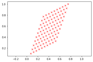
Example:: Apply an affine transform to a uniform grid.

from afbf import coordinates
from numpy import array

coord = coordinates(10)
coord.Display(1)
A = array([[1, 3], [2, 1]], dtype=int)
coord.ApplyAffineTransform(A)
coord.Display(2)

CheckValidity()

Check the validity of coordinates.

Returns:: True if attributes are properly defined, and false otherwise.
Return type:: boolean

DefineNonUniformLocations(xy)

Import a set of positions provided in an array.

Parameters:: xy (ndarray) – An array of size (ncoord, 2) containing coordinates: xy[m, :] are the mth coordinates.
Returns:: Attributes xy, M, N, grid.
Example:: Define coordinates at some given positions.

from afbf import coordinates
from numpy import array

xy = array([[1, 2], [3, 4], [-2, 2], [5, 6]], dtype=int)
coord = coordinates()
coord.DefineNoneUniformLocations(xy)

DefineSparseSemiBall(N, step=1)

Define a sparse semi-ball.

Parameters:: N (int) – number of x- and y- coordinates.
Returns:: Attributes xy, N, Nx, Ny, grid.

DefineUniformGrid(N, step=1, signed=False)

Define a uniform grid.

Parameters:

N (int) – number of x- and y- coordinates.
step (int, optional) – step between grid points. Default to 1.
signed (boolean, optional) – True if the grid is to be signed.

Returns:

Attributes xy, N, Nx, Ny, grid.

Display(nfig=1)

Display the positions given by coordinates.

Parameters:: nfig (int, optional) – The index of the figure. Default to 1.

ProjectOnAxis(u, v)

Project coordinates on an axis oriented in (u, v).

Given the axis \((u, v)\) and coordinates \((x, y)\), the projection is given by

\[z = u\: x + v \: y\]

Parameters:: v (int u,) – The projection axis.
Returns:: Projection coordinates.
Return type:: ndarray of shape (ncoord, 2)

Spatial data (sdata)

class afbf.Classes.SpatialData.sdata(coord=None, name='undefined')

Bases: object

This class handles spatial data.

Spatial data includes but are not restricted to images. Images are particular spatial data defined on a uniform grid.

Parameters:

coord (coordinates) – Coordinates where data are defined.
values (ndarray) – Spatial values observed at each position of coord; values[m] is the value observed at position coord[m, :].

:param ndarray M: size of the image (number of rows, columns).

Parameters:: name (str, optional) – Name of data. Default to ‘undefined’.

ComputeEmpiricalSemiVariogram(lags)

Compute the empirical semi-variogram of an image.

Parameters:: lags (coordinates) – Lags at which to compute quadratic variations.
Returns:: The semi-variogram.
Return type:: sdata

Note

This method only applies to an image.

ComputeImageSign()

Compute the sign of an image.

Returns:: The sign image.
Return type:: sdata

ComputeIncrements(hx, hy, order=0)

Compute increments of an image.

Given some lags \((h_x, h_y)\) and an order \(J\), increments \(Z\) of order \(J\) of the image form an image defined in a recursive way by

\[\begin{split}\left\{ \begin{array}{l} X^{(0)} = X, \\ X^{(j+1)} [x, y] = X^{(j)}[x, y] - X^{(j)}[x - h_x, y - h_y], \:\: \mathrm{for} \:\: j = 0, \cdots, J, \\ Z = X^{(J+1)}. \end{array}\right.\end{split}\]

Parameters:

hy (int hx,) – Horizontal and vertical lags.
order (int) – Order of the increment. The default value is 0.

Returns:

The increment image.

Return type:

sdata

ComputeLaplacian(scale=1)

Compute the discrete laplacian of an image.

Given some scale \(s\), the Laplacian \(Z\) of the image is an image defined as

\[Z[x, y] = 4 X[x, y]-X[x-s, y]-X[x+s, y]- X[x, y-s] - X[x, y+s].\]

Parameters:: scale (int , optional) – Scale at which the Laplacian is computed. Default to 1.
Returns:: The image Laplacian.
Return type:: sdata

ComputeQuadraticVariations(lags, order=0)

Compute the quadratic variations of an image.

Parameters:: lags (coordinates) – Lags at which to compute quadratic variations.
Aram order:: The order of the quadratic variations. The default is 0.
Returns:: Quadratic variations.
Return type:: sdata

Note

This method only applies to an image.

CreateImage(M)

Create an image.

Parameters:: M (ndarray) – An array of size 2 giving the number of rows and columns of the matrix.
Returns:: Attribute coord.

Display(nfig=1)

Display an image.

Parameters:: nfig (int, optional) – Figure index. Default to 1.

ImportImage(filename)

Import an image.

Parameters:: filename (str.) – Physical address of the image.

Save(filename)

Save an image in a file

Parameters:: filename (str) – File name (without extension).

Process (process)

class afbf.Classes.RandomProcess.process(type='fbm', param=-1)

Bases: object

This class handles random processes, with a focus on fractional Brownian motions (FBM).

A FBM is a Gaussian random process with stationary increments. Its properties (regularity, order of self-similarity, …) are determined by a single parameter \(H \in (0, 1)\), called the Hurst index.

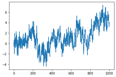
Example:: Simulation of a FBF with Hurst index \(H=0.2\) at times \(\{1, \cdots, T\}\).

from afbf import process
model = process('fbm', param=0.2)
model.Simulate(T=1000)
model.Display(1)

:param ndarray autocov: The autocovariance of the process.

:param ndarray spect: The Fourier spectrum of the autocovariance.

:param ndarray vario: The semi-variogram of the process.

:param ndarray y: The values of a simulation of the process.

ComputeAutocovariance(T=10)

Compute the autocovariance of the process increments: at uniformly-spaced lags \(\{0, 1, \cdots, T\}\).

Parameters:: T (int) – The maximal lag. Default is 10.
Returns:: Attribute autocov.

ComputeAutocovarianceSpectrum()

Compute the Fourier spectrum of the periodized autocovariance.

Returns:: Attribute spect.

ComputeFBMAutocovariance(T)

Compute the autocovariance of the increments of a fractional Brownian motion of Hurst index \(H\) at uniformly-spaced lags \(\{0, 1, \cdots, T-1 \}\).

Parameters:: T (int) – The maximal lag.
Returns:: Attribute autocov.

ComputeFBMSemiVariogram(lags, logvario=0)

Compute the semi-variogram of the fbm at lags given in lags.

Parameters:

lags (ndarray) – Lags where to compute the variogram.
logvario (int, optional) – if logvario>0, a log semi-variogram is computed. The default is 0.

Returns:

Attribute vario.

ComputeSemiVariogram(lags, logvario=0)

Compute the semi-variogram of the process at lags given in lags.

Parameters:

lags (ndarray) – Lags where to compute the variogram.
logvario (int, optional) – if logvario>0, a log semi-variogram is computed. The default is 0.

Returns:

Attribute vario.

Display(nfig=1)

Display the realization of the process.

Parameters:: nfig (int, optional) – Figure index. The default is 1.

ExtendFBM(M=5)

Extend the definition of a FBM to a non self-similar process.

Parameters:: M (int, optional) – The number of parameters used for defining the extension function. The default is 5.
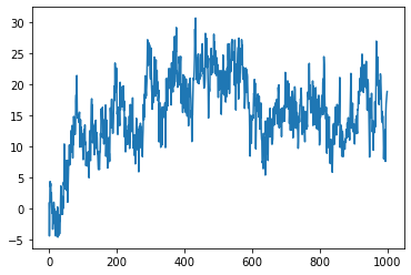
Example:: Simulation of an extended FBF with Hurst index \(H=0.2\) at times \(\{1, \cdots, T\}\).

from afbf import process
model = process('fbm', param=0.2)
model.ExtendFBM()
model.Simulate(T=1000)
model.Display(1)

IntegrateProcess(order)

Integrate the process at a given order.

Parameters:: order (int) – The order of integration.
Returns:: Attribute y.

Simulate(T)

Simulate the process at uniformly-spaced positions: \(\{0, 1, \cdots, T\}\).

Parameters:: T (int) – The maximal lag.
Returns:: Attribute y.

Simulate_CirculantCovarianceMethod(T)

Simulate process increments at positions \(\{0, 1, \cdots, T\}\).

Note

The method was developed by Wood and Chan. It is described in [14].

Parameters:: T (int) – The maximal lag.
Returns:: Attribute y.

Turning bands (tbparameters)

class afbf.Simulation.TurningBands.tbparameters(K=500)

Bases: object

This class handles parameters of the turning band field.

Parameters:

K (int) – the number of bands.
Kangle (ndarray) –
Angles of the turning bands. The tangent of each angle \(\varphi\) have a tangent which satisfies

\[\tan(\varphi) = \frac{p}{q},\]

for some \(p \in \mathbb{Z}\) and \(q \in \mathbb{N}^*\).
Pangle (ndarray) – Denominators \(q\) of angle tangents.
Qangle (ndarray) – Numerators \(p\) of angle tangents.
cost (scalar) – Angle cost (dynamic programming).
acc (scalar) – Precision (dynamic programming).

DisplayInformation(): Display information about simulation.

OptimalAngles(N=500)

Compute a set of optimal angles by dynamic programming.

Parameters:: N (scalar) – The expected precision. if \(N < 1\), the precision is set to N else the precision (in radians) is set to \(\frac{pi}{N}\).
Returns:: Attributes Kangle, Pangle, Qangle.

Note

The dynamic programming algorithm finds an optimal subset \(S'\) of angles among a set \(\Phi\) of possible angles whose tangents are rational. :math:`Phi`is a subset of

\[\{\varphi \in [-\pi/2,\pi/2], \tan(\varphi)=p/q, p \in \mathbb{Z}, q \in \mathbb{N}^\ast, p \wedge q=1\}.\]

A cost \(C(\varphi)=\vert q \vert+p\) is associated to each angle \(\varphi\).

The optimal subset \(\Phi'\) minimizes \(\sum_{\varphi \in \Phi'} C(\varphi)\) under the constraint that the difference between two successive angles are below a given precision.

Precision(): Compute the precision of the turning bands.

QuasiUniformAngles(K=100000)

Build a set of K angles which are approximately uniform on the interval \([-\frac{\pi}{2},\frac{\pi}{2}]\).

Parameters:: K (int, optional) – A number of angles. The default is 100000.
Returns:: Attributes Kangle, Pangle, Qangle.

SimulationCost(): Compute the computational cost associated to the turning bands.

ndarray

class afbf.utilities.ndarray

ndarray(shape, dtype=float, buffer=None, offset=0,: strides=None, order=None)

An array object represents a multidimensional, homogeneous array of fixed-size items. An associated data-type object describes the format of each element in the array (its byte-order, how many bytes it occupies in memory, whether it is an integer, a floating point number, or something else, etc.)

Arrays should be constructed using array, zeros or empty (refer to the See Also section below). The parameters given here refer to a low-level method (ndarray(…)) for instantiating an array.

For more information, refer to the numpy module and examine the methods and attributes of an array.

Parameters

(for the __new__ method; see Notes below)

shapetuple of ints: Shape of created array.
dtypedata-type, optional: Any object that can be interpreted as a numpy data type.
bufferobject exposing buffer interface, optional: Used to fill the array with data.
offsetint, optional: Offset of array data in buffer.
stridestuple of ints, optional: Strides of data in memory.
order{‘C’, ‘F’}, optional: Row-major (C-style) or column-major (Fortran-style) order.

Attributes

Tndarray: Transpose of the array.
databuffer: The array’s elements, in memory.
dtypedtype object: Describes the format of the elements in the array.
flagsdict: Dictionary containing information related to memory use, e.g., ‘C_CONTIGUOUS’, ‘OWNDATA’, ‘WRITEABLE’, etc.
flatnumpy.flatiter object: Flattened version of the array as an iterator. The iterator allows assignments, e.g., x.flat = 3 (See ndarray.flat for assignment examples; TODO).
imagndarray: Imaginary part of the array.
realndarray: Real part of the array.
sizeint: Number of elements in the array.
itemsizeint: The memory use of each array element in bytes.
nbytesint: The total number of bytes required to store the array data, i.e., itemsize * size.
ndimint: The array’s number of dimensions.
shapetuple of ints: Shape of the array.
stridestuple of ints: The step-size required to move from one element to the next in memory. For example, a contiguous (3, 4) array of type int16 in C-order has strides (8, 2). This implies that to move from element to element in memory requires jumps of 2 bytes. To move from row-to-row, one needs to jump 8 bytes at a time (2 * 4).
ctypesctypes object: Class containing properties of the array needed for interaction with ctypes.
basendarray: If the array is a view into another array, that array is its base (unless that array is also a view). The base array is where the array data is actually stored.

Notes

There are two modes of creating an array using __new__:

If buffer is None, then only shape, dtype, and order are used.
If buffer is an object exposing the buffer interface, then all keywords are interpreted.

No __init__ method is needed because the array is fully initialized after the __new__ method.

Examples

These examples illustrate the low-level ndarray constructor. Refer to the See Also section above for easier ways of constructing an ndarray.

First mode, buffer is None:

>>> np.ndarray(shape=(2,2), dtype=float, order='F')
array([[0.0e+000, 0.0e+000], # random
       [     nan, 2.5e-323]])

Second mode:

>>> np.ndarray((2,), buffer=np.array([1,2,3]),
...            offset=np.int_().itemsize,
...            dtype=int) # offset = 1*itemsize, i.e. skip first element
array([2, 3])

API: auxiliary classes

Periodic functions (perfunction)

Coordinates (coordinates)

Spatial data (sdata)

Process (process)

Turning bands (tbparameters)

ndarray

Parameters

Attributes

See Also

Notes

Examples