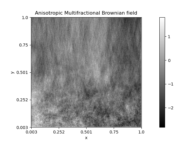
Anisotropic Multifractional Brownian field 2

Code author: Frédéric Richard <frederic.richard_at_univ-amu.fr>

In this example, we show how to simulate heterogeneous textures whose anisotropy spatially varies. Such textures can be obtained by simulating a turning band field with a space-dependent Hurst function represented as a step function.

Here, the Hurst function \(\beta_{(x,y)}\) is defined at position \((x, y)\) by changing linearly a Hurst constant. The directional properties of the generated texture vary in the vertical direction from anisotropic to isotropic while its roughness remains the same.

Note

Such simulations are related to the so-called anisotropic multifractional Brownian field which was investigated [8]. In a harmonizable representation, these fields are defined as

\[Z(x, y) = \int_{\mathbb{R}^2} (e^{i\langle (x, y), w \rangle} -1 ) \tau_{(x, y)}(w) \vert w \vert^{-\beta_{x, y}(w) -1} dW(w),\]

where \(dW\) stands for a complex Brownian measure.

import numpy as np
from afbf import coordinates, sdata, tbfield

N = 256  # Image size.

pid = np.pi / 5  # length of a step of the Hurst function.
dpid = np.pi / 16  # length of the transition between steps.

h0 = 0.1  # Hurst index at (x, y) with y=0.
h1 = 0.9  # Hurst index at (x, y) with y=N-1.

pid = np.pi / 16  # length of a step of the Hurst function.
dpid = np.pi / 6  # length of the transition between steps.
h0 = 0.1
h1 = 0.9

# Define a field.
Z = tbfield('afbf-smooth')
# Set step interval bounds.
Z.hurst.ChangeParameters(
        np.array([[h1, h0]]),
        np.array([[-pid - dpid, -pid, pid, pid + dpid]])
    )
Z.hurst.trans = 1  # Indicate where step transitions are.

# Set coordinates.
coord = coordinates(N)  # field coordinates.
coordy = coordinates()  # subset of coordinates.
x = np.reshape(np.arange(1, N+1), (N, 1))

# Initialize an image.
z = sdata(coord)
z.name = 'Anisotropic Multifractional Brownian field'

for y in range(N):
    # Rescale the Hurst function.
    t = y / (N - 1)
    h = h0 * t + h1 * (1 - t)
    # Change the step constants.
    Z.hurst.ChangeParameters(
        np.array([h, h0])
    )
    # Normalization.
    Z.NormalizeModel()

    # Restrict to coordinates (:, y).
    coordy.DefineNonUniformLocations(
        np.concatenate((x, (y+1) * np.ones((N, 1))), axis=1))
    coordy.N = coord.N

    # Simulate the current field keeping a same random seed.
    np.random.seed(1)
    zy = Z.Simulate(coordy)

    # Keep the simulation at positions  (y:-1, :).
    z.values.reshape(N, N)[y, :] = zy.values.reshape(1, N)[0, 0:N]

# Display the simulation.
z.Display()